
2D Or Not 2D:
Bridging the Gap Between Tracking
and Structure from Motion
Karel Lebeda, Simon Hadfield and Richard Bowden.
Overview
The aim of our TMAGIC (Tracking, Modelling And Gaussian-process Inference Combined) tracker is to track an a priori unknown object (i.e. to determine its trajectory) in every frame of a video-sequence, given only its initial position. In other words, our algorithm has a video as an input and an object of interest specified by a bounding box in the first frame: no further human supervision is provided. The primary output from the tracking point of view is then the location of the target in every consecutive frame of the video. This trajectory can then be used in further applications such as behaviour analysis, area monitoring or object stabilisation (for recognition, super-resolution etc.).
In order to correctly handle changing viewpoints, we model the target as a 3D object in a 3D world. Therefore, the trajectory we estimate is not only in 2D (X-Y location in the video), but also as a full 3D pose, relative to the camera (X-Y-Z location and roll-pitch-yaw rotation, a.k.a. 6 degrees of freedom). The 3D model used by the tracker can be exported and used as one of the outputs. Possible applications are numerous, in, for instance, robotics (navigation and manipulation), virtual and augmented reality, 3D printing or the entertainment industry (2D film uplifting or bringing real-world assets into virtual worlds).
For the purposes of our tracker, the 3D shape of the object is modelled as a Gaussian Process. This allows a fully probabilistic inference, robust to overfitting and providing confidence measure on every point of the object surface.
Motivation
Visual tracking is a relatively old and developed area. One of the major challenges researchers in the area have been trying to tackle is changing appearance of the tracked target over time. This can have several reasons, e.g. varying illumination or viewpoint. While previous works on the topic were handling changing viewpoint (also called out-of-plane rotations) by learning different appearance from different angles, we have decided to model it explicitly.
This gives our approach several advantages against conventional (2D) trackers. Firstly, it does not need to learn new appearances when the object don't actually change (this prevents the model from drifting away from reality). Secondly, it can handle even very fast out-of-plane rotations, where state-of-the-art 2D trackers fail to adapt rapidly enough (see the Rally-VW video below for a rotation by almost 180 degrees in less than 100 frames). Finally, the 3D internal representation leads to much richer outputs. The 2D trajectory is not supplied only as a location or a bounding box, but as a coarse object-background segmentation. The trajectory can also be returned directly in 3D, opening many new possibilities. The last, but by no means least, is the 3D model with even more uses than the trajectory itself.
Method
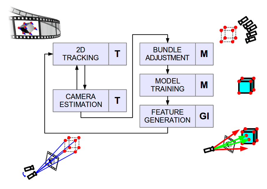
The diagram above shows the overview of the TMAGIC flow. The algorithm consists of two main loops. The tracking loop is performed on every frame and consists of tracking 2D features and then estimating the camera pose. Once the camera moves by a significant amount, the modelling loop is started, consisting of an iterative optimisation of our 3D feature cloud and camera trajectory, retraining of the surface shape model and finally of generation of new features. The letters next to the blocks illustrate which part of the algorithm they relate to - Tracking, Modelling or Gaussian-process Inference.
Without a fixed reference frame of the 3D world, there is no difference between movement of the object and of the camera. Only relative motion is perceived. See, for instance, the Cube video, where we cannot unambiguously decide if the cube is rotating, or the camera circling around. Therefore we can use object-centric system and without loss of generality assume that the object is static and the camera is moving around it.
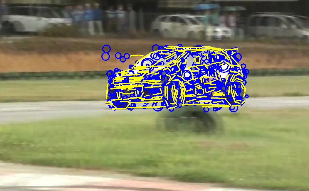
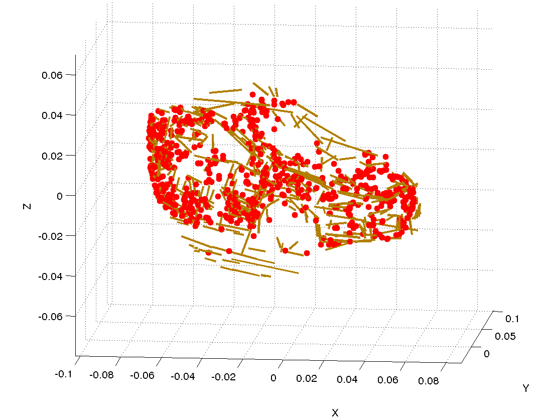
In this work we use so-called features, i.e. small, locally distinctive regions of the image. In our work we use standard point features and also line-segment features, providing additional information e.g. for low-textured objects where point features are scarce. We use the term 2D features for features located in particular time on particular locations in the video. Their (reconstructed) physical counterparts in the 3D world are then called 3D features (see the examples above). We say 3D and 2D features are in correspondence when 2D feature is a projection (image) of the 3D feature. Our 2D features are tracked independently on a frame-to-frame basis. From the new (tracked) 2D features and their 3D correspondences we can then estimate the position of the camera for the following frame. Concatenating the camera poses gives the final 3D trajectory. The 2D trajectory (of the target object) can be provided by overlaying projection of the object shape model over every frame of the video in a augmented-reality style. This can be done on-the-fly (also called online processing), i.e. for any given frame the partial output can be returned before the next frame is provided.
In the modelling loop, first a Bundle Adjustment is run. That takes all our features (2D in all frames and 3D) together with the camera trajectory into one joint iterative optimisation and refines the camera trajectory and the 3D feature positions in order to fit the 2D feature observations with their expectation. Ceres Solver is employed in this task. Using the refined feature cloud, our surface shape model is retrained (see the video below). Finally, new features are created such that they represent distinctive areas in the image frame and at the same time belong to a region of low confidence on the object surface. This is one of the major uses for the Gaussian Process model.
Results
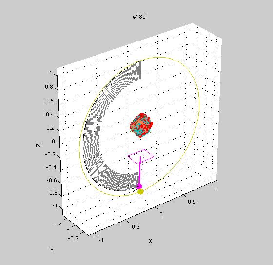
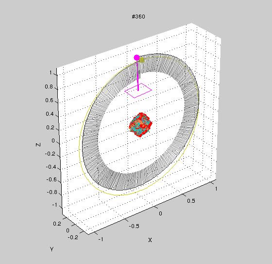
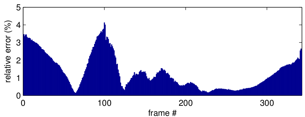
We firstly tested the TMAGIC tracker on the synthetic sequence Cube to measure its performance quantitatively. The perfect shape is, obviously, a cube, and the ideal trajectory is a circle around its centre stepping with speed of one degree per frame. As you can see from the graph below, the deviations from the perfect circular trajectory are in order of percents, which is significantly better than state-of-the-art reconstruction toolkits such as VisualSFM, with comparable reconstruction accuracy (fit of the model to a perfect cube).
To compare against state-of-the-art 2D trackers, we evaluated them as well as TMAGIC on several real-world sequences, including both previously published ones and new ones. As can be seen from the charts below, it outperforms conventional trackers, especially in cases of strong out-of-plane rotations (second row of images). The sequences are, from the top and left, Dog, Fish, Sylvester, Twinings, Rally-Lancer, Rally-VW, TopGear1 and TopGear2. TMAGIC always scores among the best and on most sequences it is the very best one. On reviewers' request, we measured mean overlap of bounding boxes besides the localisation error, however our conclusions stay unchanged. See the paper for a table with full results.
Publications
K. Lebeda, S. Hadfield and R. Bowden:
2D Or Not 2D: Bridging the Gap Between Tracking and Structure from Motion.
In Proc. of ACCV, 2014.
Download:
<pdf>,
<bib>,
<poster>,
<presentation (PRCVC)>,
<data and results>.
This work loosely follows our previous publications on visual tracking:
K. Lebeda, S. Hadfield, J. Matas and R. Bowden:
Long-Term Tracking Through Failure Cases.
In Proc. of ICCV VOT, 2013.
Download:
<pdf>,
<bib>,
<data>,
<presentation>,
<poster (BMVA TM)>.
K. Lebeda, J. Matas and R. Bowden:
Tracking the Untrackable: How to Track When Your Object Is Featureless.
In Proc. of ACCV DTCE, 2012.
Download:
<pdf>,
<bib>,
<data>,
<poster>,
<presentation>.
Acknowledgements
This work was part of the EPSRC project “Learning to Recognise Dynamic Visual Content from Broadcast Footage” grant EP/I011811/1. Its presentation has been supported by the BMVA student Travel Bursary. The (LT-)FLOtrack publications were also supported by the following projects: SGS11/125/OHK3/2T/13, GACR P103/12/2310 and GACR P103/12/G084.
